Software and Downloads
Please check out our GitHub repository. New code will be released on GitHub. Most
of the downloads found on this page have migrated to GitHub and might not get
updated here.
Contents
Plotting Atomic Orbitals (AOs) with Mathematica
Plotting Molecular Orbitals (MOs) with Mathematica
Plotting rank-2 tensors
Manipulate CUBE format volume data files
Crystal field Hamiltonian and atomic shell splitting
PNMRShift: A software tool for NMR shifts of paramagnetic molecules
KK-GUI: Software with graphical interface to perform Kramers-Kronig
transformations
CD spectra toolkit
Template for plots of spectra (or other stuff) with Gnuplot and LaTeX
______________________
Plotting Atomic Orbitals (AOs) with Mathematica
(explore on GitHub)
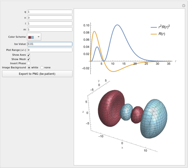
You can use this notebook to visualize the orbitals (wavefunctions) of hydrogen-like
atoms. The plot interface is shown above, along with visualizations of a 3px
hydrogen orbital. For non-zero values of the magnetic quantum number m, the usual
real ’sine’ and ’cosine’ linear combinations are created for -/+m.
______________________
Plotting Molecular Orbitals (MOs) with Mathematica
(explore on GitHub)
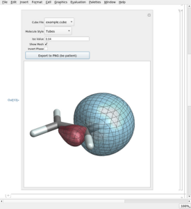

Rather: Plotting isosurfaces of molecular orbitals... Please follow the link to GitHub
shown above, then follow the links that mention orbital plotting, to see detailed
descriptions and download options. The notebooks use volume data in the popular
cube format.
______________________
Plotting rank-2 tensors
(explore on GitHub)

A Mathematica notebook for plotting graphical representations of NMR shielding
tensors; easily adaptable for other types of rank-2 tensors (EFG, Optical Rotation,
and others).
Description and some examples
Download the Mathematica (v. 12 and higher) notebook (60 kByte)
Here is the notebook for older Mathematica versions (up to v. 11) (52 kByte)
Download an XYZ molecular coordinate file read by the notebook (16 kByte)
If you use this plotting tool for your research, please cite the recommended references
given at the top in the notebook.
______________________
Manipulate CUBE format volume data files
See the repository on on GitHub. manipulatecube is a Fortran tool used by me and
my group to work with volume data files in the ’Gaussian cube’ format.
You can use manipulatecube to multiply the volume data by a factor and
integrate the cube, take linear combinations of two data sets (same grid, same
molecule), add or multiply two cube files (same grid, same molecule), or
use manipulatecube to bring a data set for an orthogonal but unsorted
(not in the order x, y, z) grid, or a grid with negative steps (going from
positive to negative coordinate values), into a more standard grid format.
[Not all of the available visualization software packages can handle grids
with negative steps or grids with vectors that aren’t in the order of x, y, z
direction].
______________________
Crystal field Hamiltonian and atomic shell splitting
(explore on GitHub)

A Mathematica notebook for the symbolic calculation of a crystal field Hamiltonian and
the spin-orbit coupling Hamiltonian in a basis of atomic orbitals for a given angular
momentum ,
along with other calculations.
Description and some examples
Downloads the Mathematica notebook (792 kBytes)
______________________
PNMRShift: A software tool for NMR shifts of paramagnetic molecules
(explore on GitHub)

Here you can download the source code along with Linux and Windows (32 bit)
binaries of a program that reads calculated magnetic resonance tensors (Ramsey
shielding, EPR Zeeman and hyperfine coupling), and optionally zero-field splitting,
and assembles chemical shift tensors for a given temperature and pseudo-spin. For
details see Reference [224]
Download PNMRShift (4.2 MByte. GPL)
______________________
KK-GUI: Software with graphical interface to perform Kramers-Kronig
transformations
(explore on GitHub)
This software is useful if you have absorptive or dispersive spectral data and want to
perform a Kramers-Kronig (KK) transformation to obtain the dispersive /
absorptive counterpart. Works under Linux and Windows and comes in two
versions that are both included in the package. Both versions are written
in Python and use the Python interface with Tcl/Tk and Matplotlib for
the GUI and the resulting plots. One version includes numerical routines
in Fortran that need to be compiled. The second version is Python-only
and does not require a compiler, but its KK transformations are slower. It
is possible to perform ‘anchored’ KK transformations known as multiply
subtractive KK (MSKK) or chained doubly-subtractive KK (CDKK); these
methods are described in Reference [92]. KK-GUI was developed in 2017 by
Mr. Herbert Ludowieg, then an undergraduate research assistant in my group,
based on prior developments by Mark Rudolph, Patrick Dawson, and Mikhail
Krykunov.
Download KK-GUI (458 KByte. GPL)
Below is a screen shot of the interface. We loaded optical rotatory dispersion data
(red curve) into the software and let it generate the corresponding circular dichroism
spectrum (blue curve).

______________________
CD spectra toolkit
Note: Our spec-gen Python script provides much of the functionality of the old CD
spectra toolkit, which is therefore no longer maintained.
Here you can download a package containing some Unix shell scripts and the
Fortran source code for two programs. Compiled binaries for a 32 bit Linux system
are included. The Fortran source code should compile with any f90 compiler. Please
email me if it doesn’t.
Download gzipped tar archive (781 kByte)
Together the scripts and programs process the output of a time-dependent DFT CD
spectrum calculation and generate a nice simulated spectrum. The CD spectrum can
be calculated with ADF or with Turbomole. The parsers are easily adapted for
other programs. Please see the included README file for instructions. You
need gnuplot to generate the spectra. Here is an example from Reference
[17]:

Simulated CD spectrum of [Co(en)3](3+)
______________________
Template for plots of spectra (or other stuff) with Gnuplot and LaTeX
Here is a collection of scripts and instructions (tar format, 172K) to create plots of
spectral data or similar types of scientific plots with Gnuplot and LaTeX. A
description is provided here. Below is an example of the type of plots one can make
with this script collection.
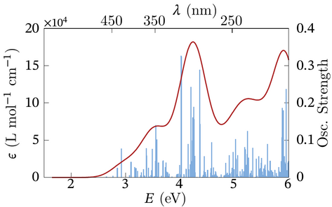
The CD spectra toolkit contains Gnuplot scripts with similar functionality, but
they were not designed to be used with the epslatex terminal of Gnuplot. The
latter was used to generate the plot above.
______________________
© 2013 – 2025 J. Autschbach. Some of the material that can be downloaded on
this web page and the associated GitHub repository is in parts or wholly based on the
results of research funded by grants from the National Science Foundation [NSF,
grants CHE 0447321, 0952253, 1265833, 1560881, 1855470, 2152633, 2503332], the
US Department of Energy (Basic Energy Sciences, Heavy Element Chemistry
program, grant DE-SC0001136), and educational activities associated with these
projects. Any opinions, findings, and conclusions or recommendations expressed in
this material are those of the author and do not necessarily reflect the views of these
funding agencies.