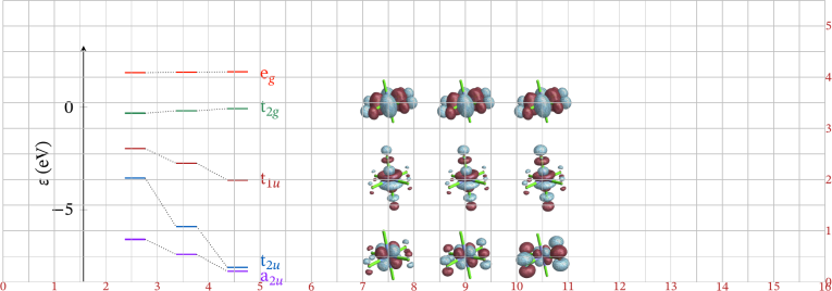
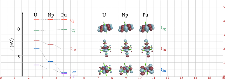
 with An = U (uranium, left), Np (neptunium,
center), and Pu (plutonium, right). Labels U, Np, Pu in black front are
given above each orbital level diagram. To the right of the diagram are
labels identifying different sets of orbitals as being of symmetry (top to
bottom) eg, t2g, t1u, t2u, a2u. The symmetry labels and the horizontal bars
indicating the orbital energy are color coded in the same way. The orbital energy
diagrams with the energy axis form the left half of the compound figure. In
the right half is a 3x3 grid of molecular orbital isosurface plots, with lobes
colored in red/blue. In each of the isosurface graphics, one can discern a
’tubes’ representation of the relevant octahedral complexe. The column
headers are U, Np, Pu. The row labels are given to the right as t2g, t1u,
t2u.](./panel-step-06.png)
In my (Jochen’s) field of science, it is often necessary to combine many different kinds of graphics into single figures with sub-panels and added labels, arrows, or other items. These kinds of figures are then used in research publications or proposals, for conference presentations or posters, or on a web page. An example for such a figure is this
Furthermore, to avoid making silly looking figures (e.g., figures with much too large labels) for journal publications or books, it is usually a good idea to create graphical material in a specific target size, with matching font sizes being not too small and not too large. [Credit to Szabolcs Horvát, the author of the excellent ‘MaTeX’ package for Mathematica, who made a good case for designing figures in the correct size (see MaTeX documentation).] Sometimes, we need to create labels in such figures that would normally require some kind of equation editor. After weighing the pros and cons of various ways to create such figures, I have settled (after more than 2 decades of trying different things) on an approach using LaTeX. To be clear, the procedure outlined here is about making stand-alone PDF files of appropriately sized and labeled compound figures. These PDFs can be included easily in a LaTeX manuscript but also in a word-processing software of your choice. (See the end of this page for format conversion tips.)
For example, I recently needed to make a figure combining a molecular orbital (MO) diagram with several MO visualizations (as isosurface plots) and assorted labels, like the one shown above. The MO visuals were generated with a separate software in comparatively high resolution (on the order of 1500x1500 pixels in the example). Specifically, these images were generated in PNG format with one of my Mathematica notebooks, using volume data files for the different MOs that were created based on calculations with a quantum chemistry program package. However, such isosurface plots can be created with a large variety of software packages, open-source or proprietary.
In this archive (tar format, 9MB), in directory plots/, there is a file
panel-mo-diagram-and-orbitals.tex used to assemble the various graphical
objects and labels, and a shell script make-panels.sh to compile the figure with
xelatex. There is furthermore a file 10-modiagram.tex that is first compiled by
the script to prepare the MO diagram, which is subsequently included in
panel-mo-diagram-and-orbitals.tex. Both LaTeX files can also be
compiled individually with xelatex, which is useful during the trial & error
period of designing the combined figure. The script is written such that
tex files with names starting with a double-digit number (01, 10, 23, 99)
get compiled first, in the order of numbering, and then tex files whose
names start with panel- get compiled subsequently in the order of how your
system sorts them in a file listing. This was done so that dependencies of a
given panel are reliably compiled first. The script will stop whenever there
is an error encountered. LaTeX errors will be listed in the resulting .log
files.
Before you try out this example, please make sure you have a working TeX
distribution with xelatex and STIX2 (or STIXTwo) and various other font sets, and
Ghostscript. If you can successfully compile my article template posted here
(direct download), you should be good to go as far as font installations
are concerned (or switch to default fonts). To compile the panel example,
your TeX installation also needs a variety of utility packages such as tikz
and pgfplots. As a Linux user, I usually install a TeX Live distribution
including all packages on my systems. Other TeX distributions have similar ‘full’
installation options. (Who cares about a few GB of extra disk space usage these
days?)
In each tex file in the archive, not far below \begin{document} there is
code to set the size of the plotting canvas in centimeters. For example, in
panel-mo-diagram-and-orbitals.tex we set the figure canvas initially to be 16
cm wide and 5.5 cm high. This is a suitable size for a figure that would span up to
two columns in a typical scientific journal. The code is
\setlength{\mx}{16cm}
\setlength{\my}{5.5cm}
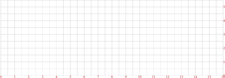
This can be adjusted, of course. Next, closer to the end of the file there is some code that will create a grid with 0.5 cm spacing the size of the canvas specified earlier, which you can use later to aid placement of images, labels, and so on. Using
% Grid to help placing objects, if so requested
\renewcommand{\showgrid}{true} % use true or false
with a value of true draws the grid. Set to false and recompile, and the grid will
not be shown. Note that with the standalone documentclass, the resulting figure
will be cropped automatically, so if the grid extends beyond any of the drawing
elements then the figure without the grid will be smaller than the canvas size
specified.
Without having anything placed in the panel, with \showgrid set to true, the
panel (after compiling panel-mo-diagram-and-orbitals.tex with xelatex looks
like this:
The LaTeX code for the MO diagram is kind of complicated (though relatively
easy to use) and was put together with the help of many posts on Stack Exchange.
It has an initial canvas setting of 8.5 x 5 cm but ends up being smaller
than that after the grid is removed. Since we are creating the figure in the
intended size, with matching font sizes, the MO diagram does not need to be
scaled when it is included in the panel. After it has been compiled into a
PDF, we include it in panel-mo-diagram-and-orbitals.tex with the
code
% orbital level plot:
\node[above right] (image) at (0.5,0) {
  \includegraphics{10-modiagram}
};
The .pdf file name extension is not required for xelatex, but make sure the PDF
is the only graphics version of the MO diagram, unless you are sure that the PDF
version would be included even if a PNG or some other format version is present. I
note in passing that JPEG is not a good format for line drawings such as function
graphs or MO diagrams and other types scientific graphics that tend to have a lot of
white space and even colors. Anyhow, the resulting compiled panel now looks like
this:
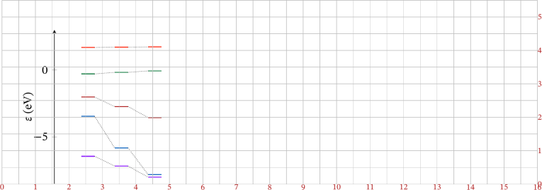
(Of course, one can draw the MO diagram with a different software and include
the resulting image file in the panel instead.) Next, we place symmetry labels for the
MO levels in the diagram. The color specs and the macros \ttwog (typeset:
)
etc. are defined in the tex files. I forgot why there is a \strut in each of the labels
but it has to do with the placement and the vertical extension of the box holding the
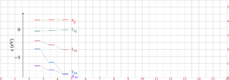
label. We add the code
\node[right] at (5,4.05){\strut \orange{\eg{}}};
\node[right] at (5,3.4){\strut \green{\ttwog{}}};
\node[right] at (5,2){\strut \red{\toneu{}}};
\node[right] at (5,0.4){\strut \blue{\ttwou{}}};
\node[right] at (5,0.1){\strut \purple{\atwou{}}};
The coordinates used in those commands correspond to the location within the grid that we drew on the canvas. The panel now looks like this:
Next, we place a set of nine MO isosurface images, using
% orbital plots
\node (image) at (7.5,3.5) {
  \includegraphics[scale=0.1]{U_t2g_ADF}
};
\node (image) at (9,3.5) {
  \includegraphics[scale=0.1]{Np_t2g_ADF}
};
\node (image) at (10.5,3.5) {
  \includegraphics[scale=0.1]{Pu_t2g_ADF}
};

\node (image) at (7.5,2) {
  \includegraphics[scale=0.1]{U_t1u_ADF}
};
\node (image) at (9,2) {
  \includegraphics[scale=0.1]{Np_t1u_ADF}
};
\node (image) at (10.5,2) {
  \includegraphics[scale=0.1]{Pu_t1u_ADF}
};

\node (image) at (7.5,0.5) {
  \includegraphics[scale=0.1]{U_t2u_ADF}
};
\node (image) at (9,0.5) {
  \includegraphics[scale=0.1]{Np_t2u_ADF}
};
\node (image) at (10.5,0.5) {
  \includegraphics[scale=0.1]{Pu_t2u_ADF}
};
The relative location of these PNG image files is directory ../share/ (the naming
is for compatibility with our texcollab utility). Instead of adding the file path in the
\includegraphics commands directly, directory ../share/ is specified in the
definition of \graphicspath in the panel tex file, so the files are found by LaTeX
without an explicit path specification. After compiling, the panel looks like
this:
Add some more labels,
\node[right] at (11.5,3.5){\strut \green{\ttwog{}}};
\node[right] at (11.5,2){\strut \red{\toneu{}}};
\node[right] at (11.5,0.5){\strut \blue{\ttwou{}}};

\node at (2.5,4.4){\strut U};
\node at (3.6,4.4){\strut Np};
\node at (4.55,4.4){\strut Pu};

\node[right] at (7.3,4.4){\strut U};
\node[right] at (8.7,4.4){\strut Np};
\node[right] at (10.2,4.4){\strut Pu};
and the panel looks like this:
Finally, we remove the grid by setting
% Grid to help placing objects, if so requested
\renewcommand{\showgrid}{false} % use true or false
and recompile. The panel is now complete. When you create the figure with the
shell script make-panels.sh, the embedded high-resolution images in the resulting
PDF get downsampled to 800 DPI in the ghostscript (gs) step, which is usually
more than sufficient and tends to make the PDF a lot smaller in case there are
multiple high-resolution bitmap images included. The xelatex command
to create the initial PDF uses the -z3 option, which creates a PDF that
is not well compressed but runs much faster than xelatex with default
settings.
We sometimes have ten or more such panels for a single publication (incl. SI), and
make-panels.sh can be used to compile them all in one go (e.g., to make sure
that all compound figures are up-to-date) without waiting too long. Having
downsampled embedded images also helps to speed up scrolling through the
manuscript PDF during editing. The final version of the panel, shown near
the top of this page, is only about 11.5 cm wide without the grid, after
it’s been cropped. Most journals would still use a 2-column layout for the
figure.
The PDFs created as described here can be included easily in a LaTeX manuscript, of course. I much prefer this approach over using a gazillion of commands to produce complicated figures directly within a manuscript’s LaTeX code, although that is of course an option. You can also use the figures created as described here for inclusion in a document written with a word processor. For this, I usually convert to appropriately sized PNGs with a command such as
f="figure-file-name-without-.pdf-extension"; pdftoppm -r 600 -png ${f}.pdf > ${f}.png
The pdftoppm command is part of the poppler package available for many Linux
distributions (package naming varies). Presumably, you can also install it easily in a
Linux subsystem on Windows or on a Mac.
Final note: The tikz and pgfplots LaTeX packages are very versatile, so you can
use them to draw a lot more complicated things in your figures than just textual
labels. In research, time is of the essence, so I usually end up combining
different graphics from different sources instead of attempting a solution
using only LaTeX with tikz and/or pgfplots, say. What I described on
this page is a—better, I would argue—replacement for what people usually
end up doing, which is placing different graphics on a Powerpoint slide,
adding labels and other graphical elements, and exporting the slide as a
figure.
© 2025 – 2025 J. Autschbach.